Sometimes in my Data Science projects I need a quick and easy way to measure and visualize a predictive trend for several independent variables. My go to way to do this is to use Weight of Evidence and Information Value. Recently I put together some code in python to calculate these values and wanted to show how you can leverage these concepts to learn more about the relationship between your independent and dependent variables. These measures certainly aren’t perfect but I think they are an underutilized technique in the exploratory data analysis field.
What is Information Value and Weight of Evidence?
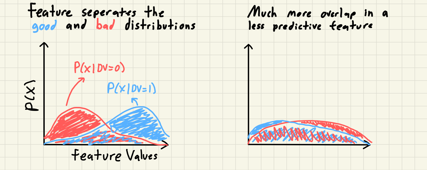
Information Value (IV) is a way to measure the strength of relationship between a feature and a dependent variable (DV). Weight of Evidence (WOE) is an individual bin’s or category’s logged risk ratio. I can’t find any information online about the history of it’s development but I first encountered this concept working at Equifax and have mostly seen resources online from banking and risk modeling. The intuition behind IV is simple; a feature that seperates the distribution of the outcomes of DV is a predictive feature that, all else being equal, you should prefer over a feature that doesn’t. This is typically discussed with a binary DV where we use the distribution of the different labels of the DV, referred to as goods vs bads. We can see this visually if we look at two hypothetical features and the distribution of the DVs within each feature.
Although interestingly you will commonly read descriptions of Weight of Evidence referring to “the distribution of goods and bads” in your DV. But really we are measuring the distribution of the feature for each seperate population of the DV labels. To do this we group our feature into bins and then calculate the percentage of goods and bads in each bin; again essentially creating a histogram of the feature for the good and bad population using consistent bin edges. Once we have our two distributions we can actually get to calculating the IV. The formula for WOE and IV is always shown as follows:
\begin{align} WOE_i = \ln(\frac{good_i}{bad_i}) \\ IV = \sum_{i=1}^N WOE_i * (good_i - bad_i) \end{align}
where $good_i$ and $bad_i$ is the percentage of the overall goods and bads in each feature bin. We can see this visually from our previous example with another poorly drawn picture:
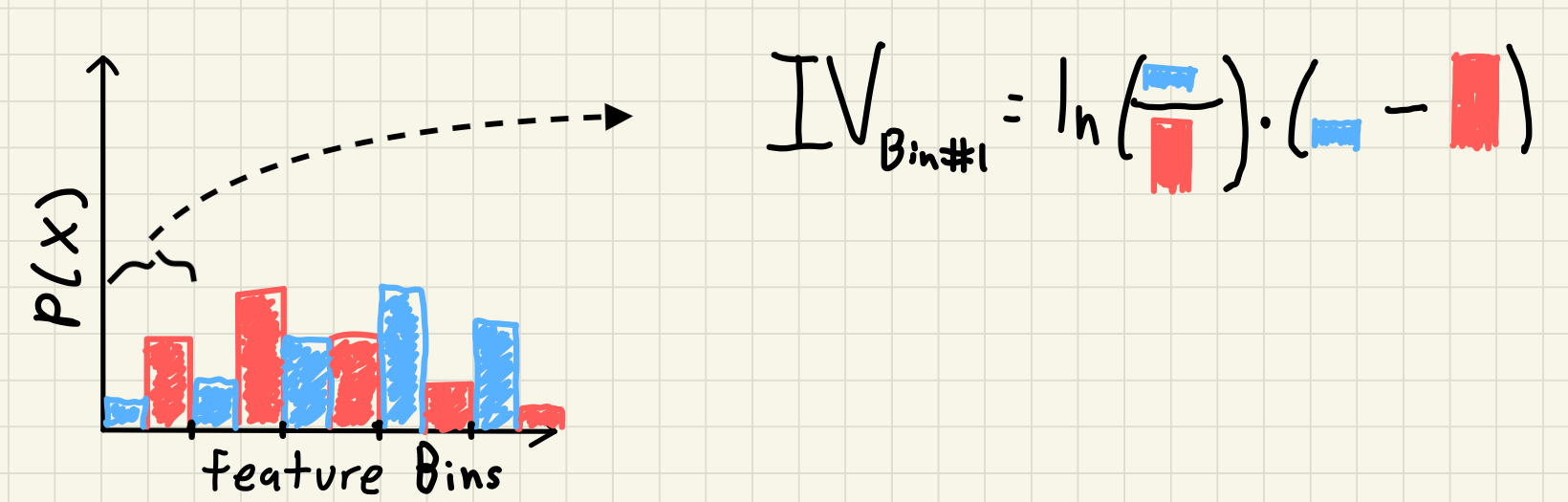
Our previous continuous distributions have been binned, and then for each bin we take the product of the ratio of the WOE and the difference in the two probability distributions.
If a feature bin has the same percentage of overall goods and bads (e.g. the lowest bin contains 25% of the overall goods and 25% of the overall bads) then that bin will have a WOE of 0 ($\ln(1) = 0$). If a feature has no seperation of goods and bads in any bin then the overall Information Value is also 0; the feature has no predictive power using this measure.
Pros and Cons of using Information Value
There are three main reasons that I prefer to use Information Value as a measure of predictiveness to compare different features over other methods:
- You can calculate IV for both numeric and categorical features and compare them across feature types. With a numeric feature we first bin the data into groups and after that we can use the exact same code as if we were calculating WOE for categorical bins.
- Missing values are handled automatically and can be treated as if
they were a seperate category. In Python we just need to ensure that
none of the steps are dropping them silently
(e.g.
groupby(..., dropna = False)). This also has the added benefit of giving you information about potentially imputing missing values. - Low frequency categories have low impact on the variable’s Information Value. If you look at the formula for Information Value we can essentially treat the term for the difference in the percentage of goods and bads in a group as a “weight” on the WOE. If we rewrite our formula from before that used $good_i$ and $bad_i$ as the overall percentage of each label in the bin to now use the number of observations in each bin, $n_i$, and the bin specific $p(bad)_i$ as the percentage of observations in each bin that are bad we can see this weighting directly.
\begin{align}
bad_i = \frac{n_i * p(bad)_i}{n_{bads}} \
good_i = \frac{n_i * (1 - p(bad)_i)}{n_{goods}} \
IV = \sum_{i=1}^N WOE_i * (\frac{n_i * (1 - p(bad)_i)}{n_{goods}} - \frac{n_i * p(bad)_i}{n_{bads}}) \
IV = \sum_{i=1}^N WOE_i * \frac{n_i}{n_{goods} * n_{bads}} * (n_{bads} - p(bad)_i * (n_{bads} + n_{goods}))
\end{align}
Honestly this last term is quite ugly but it does tell us a few things:
- As the size of the bucket, $n_i$, decreases the information value contribution for this bin also decreases
- The information value for a feature is influenced by how balanced the overall labels are but an individual bin’s IV only changes with the number of obs in the bin and how large or small the $p(bad)_i$ term is
We can also calculate an example directly to see the different contributions of four hypothetical categories; 2 rare categories and 2 more common categories with each size having one informative feature and and one with less seperation of the DV.
| Category Label | % of obs | % of goods | % of bads | WOE | Relative Diff | IV |
|---|---|---|---|---|---|---|
| Cat 1 | 1% | 1.1% | 0.9% | 0.20 | 0.002 | 0.0004 |
| Cat 2 | 1% | 2% | 0.5% | 1.39 | 0.015 | 0.021 |
| Cat 3 | 10% | 11% | 9% | 0.20 | 0.02 | 0.004 |
| Cat 4 | 10% | 20% | 5% | 1.39 | 0.15 | 0.201 |
Cat 2 has the same good to bad ratio as Cat 4 but 1/10th the contribution to the feature’s Information Value statistic because it only has 1/10th of the observations.
Of course no method is perfect and without it’s tradeoffs. Here are some of the main drawbacks to using WOE and IV as measures of feature predictiveness:
- Binning your numeric values can cause you to lose some predictive power in your feature. There are many sources that have written on this but I would recommend starting with Frank Harrell’s data method notes
- The number of bins to group your numeric features into or the max number of categories to consider is a parameter that you need to pick and could impact the value and relative rank of Information Value for different features. You could run some bootstrap simulations to quantify how big of an effect this might cause in your specific datasets.
- If either distribution of goods or bads in a bin is exactly 0 then you will receive divide-by-0 errors. To correct this I add a small bit of noise to each bin’s distribution but this may result in strange results if your bins are too small or the outcomes are too rare.
- This measure does not tell you anything else about your feature such as its correlation with other variables and whether it is fit to be included in your model.
As an exploratory measure I think that Information Value is still worth using even with these faults but one could easily argue differently.
Connection to Information Theory
A good question to ask is where did this formula come from? Why do you take the natural log of the ratio of goods and bads, but not the difference? What if you put the bads in the numerator and subtract the goods away? Luckily people smarter than me have shown that the Information Value is an equivalent expression of the symmetric KL-Divergence measure of two distributions:
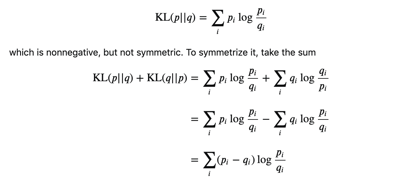
The KL-Divergence is grounded in information theory and is a common measure of how dissimilar two distributions p and q are. This way it really doesn’t matter if you use the distribution of goods first or last, you would get the same value either way.
Extension to Continuous DVs
Most explanations online only go over the use case where you are trying to predict a binary DV. If we have a continuous DV then we need a way to adopt the WOE calculation with two distinct populations to compare like we did with goods vs bads. The parallels between Information Value and the KL-Divergence gives a direction to focus on; we want a distance between a predictive and non-predictive distribution. One idea is that we can compare the distribution of our continuous DV across our feature to a baseline distribution as if the DV was evenly spread across the feature distribution. If a feature is predictive then the DV will be more concentrated in certain areas of the feature (e.g. linear feature = higher DV share at top end, quadratic = higher DV share at tails, etc…) compared to a uniform concentration for a non-predictive feature. We do have to make an adjustment to the calculations to ensure that every value of our DV is positive but WOE is scale invariant so this doesn’t change any outcomes.
Calculations in Python
I have put together a python file that can perform the full gamut of actions needed to find WOE and IV for both numeric and categorical features on my personal github. Here I will just show the code to calculate the individual WOE and IV statistics since that was the focus of the blog and to keep it short. You can view the full code here.
def calc_woe(df, feature_col, dv_col, constant = 1e-3, **bin_args):
    '''
    Calculate the WOE and IVs for the categories of the feature

    :param df: The dataframe containing the columns to use
    :param feature_col: The name of the column that contains the feature values
    :param dv_col: The name of the column that contains the dependent variable
    :param constant: The amount to add to each numerator and denominator when
                    calculating the percent of overall goods and bads to avoid
                    taking logs of 0
    '''
    df_ = df[[feature_col, dv_col]].copy()
    dv_levels = df_[dv_col].unique()

    if len(dv_levels) != 2:
        raise(f'Need only 2 levels for {dv_col}')

    num_bads = np.sum(df_[dv_col] == dv_levels[0])
    num_goods = np.sum(df_[dv_col] == dv_levels[1])

    if str(df_[feature_col].dtype) in ['string', 'category']:
        df_[feature_col + '_bins'] = trim_categories(df_[feature_col], bin_args['bins'])
    else:
        df_[feature_col + '_bins'] = bin_data(df_[feature_col], **bin_args)

    df_counts = (
        df_.
        groupby([feature_col + '_bins'], dropna = False).
        apply(lambda df: pd.Series(dict(
            num_obs = df.shape[0],
            num_bads = np.sum(df[dv_col] == dv_levels[0]),
            num_goods = np.sum(df[dv_col] == dv_levels[1])
        ))).
        reset_index()
    )

    df_counts['pct_goods'] = (df_counts['num_goods'] + min_obs) / (num_goods + min_obs)
    df_counts['pct_bads'] = (df_counts['num_bads'] + min_obs) / (num_bads + min_obs)
    df_counts['woe'] = np.log(df_counts['pct_goods'] / df_counts['pct_bads'])
    df_counts['iv'] = df_counts['woe'] * (df_counts['pct_goods'] - df_counts['pct_bads'])

    return df_counts
And here you can see a sample output of using this function on the
classic mpg dataset to predict if a car is fuel effecient or not.
mpg['fuel_effecient'] = 1.0 * (mpg['hwy'] > 30)
calc_woe(mpg, 'manufacturer', 'fuel_effecient', bins = 10)
| manufacturer_bins | num_obs | num_bads | num_goods | pct_goods | pct_bads | woe | iv |
|---|---|---|---|---|---|---|---|
| audi | 18 | 17 | 1 | 0.0454545 | 0.0801887 | -0.558302 | 0.0193921 |
| chevrolet | 19 | 19 | 0 | 0 | 0.0896226 | -4.5067 | 0.403903 |
| dodge | 37 | 37 | 0 | 0 | 0.174528 | -5.1678 | 0.901927 |
| ford | 25 | 25 | 0 | 0 | 0.117925 | -4.77849 | 0.563501 |
| other | 33 | 26 | 7 | 0.318182 | 0.122642 | 0.948375 | 0.185445 |
| hyundai | 14 | 13 | 1 | 0.0454545 | 0.0613208 | -0.29382 | 0.00466181 |
| nissan | 13 | 11 | 2 | 0.0909091 | 0.0518868 | 0.552646 | 0.0215655 |
| subaru | 14 | 14 | 0 | 0 | 0.0660377 | -4.20526 | 0.277706 |
| toyota | 34 | 26 | 8 | 0.363636 | 0.122642 | 1.08151 | 0.260639 |
| volkswagen | 27 | 24 | 3 | 0.136364 | 0.113208 | 0.184614 | 0.00427495 |
To get the full information value for this feature we just sum the individual category’s IVs.
I hope this helps some people adapt this technique in their work and analysis.